It is very important to understand that statistics deal with ONE question : if i observe a variation among a sample of N individuals ... i can compute on this sample many estimators : example for a quantitative variable : the mean m ... Then, how can i know if i'd had got the same result on another sample of N' other individuals ?
In other words, is m value (or any other estimator) due to the specific examples i chose, or is it THE mean m ? (applicable to the whole population).
In other words, are the examples set a "good" representation of the general phenomenon ?
Asking THE question of statistics in these terms allows to understand the obvious following property : if i take as a sample of the general phenomenon ALL the examples (all the possible examples, even if it is an infinite number : underlying maths idea : limit) ... then i can be sure that every estimator computed on my sample will be the estimator i would get on the whole population (by definition because in that "theoretical" case, the sample and the population tends to be the same) : i am certain of that my empirical computed estimator is THE right value..
On the contrary, if i take only ONE example (and if i assume mean of a sample of one value is the value itself), then one can understand that the computed mean i get depends entirely on the "sample" i choose ... : i am completely uncertain of that my empirical computed estimator is THE right value.
So, another way of asking ALWAYS the same question could be : how many examples should i choose in order to get a "good" value of my estimator ? (example : the mean ?).
The notion that is brought by this question is "uncertainty" : i am not sure/certain that the mean (for example) i computed on the sample is the mean (for instace) of the whole population ... Because i am interested in knowing the mean of the population (not only of the sample) than i can say that i am not certain of the mean value.
NB : However, i consider that i am sure of every value in my sample (no noise, no measurement error, ...) : uncertainty DOESN'T come from imprecision on each value : it comes from the partial observation.
If you known that your sensors have imprecision (and it is always the case), then you will have to take into account this imprecision AND the uncertainty due to the sampling effect.

---

Histogram / statistical distribution / probability

The histogram of a variable is the counting of the number of times that it takes every possible value. One uses to divide this number by the total number of examples in the sample, introducing the notion of empirical frequency distribution.
If the sample is a good representation of the total population, then empirical frequency is a way to estimate ... probability :
Example 1 : you toss a coin 10 million times (heads or tails) , and you find 4 999 999 times "reverse" (then 5 000 001 times "heads"), you can compute the empirical frequencies (about 50% 50%). If you can consider than 10 000 000 leads to a good representation of the phenomenon, then you will decide that probabilities are 50% 50%.
Example 2 : you interview 100 persons about the segment of their car : segment A (small cars), segment B (middle sized cars), segment C (big cars) and you find :

This diagram brings you information on customers.
Example 3 : case on a quantitative continuous variable (example : a length between 0 and 1)
Because the number of possible values is infinite, one uses to build a partition of the variable into small segments (ex : from 0 to 0,01, from 0,01 to 0,02, ...) in order to count the number of times the variable take a value, and then to compute the histogram.
When the number of examples tends to infinite and the segments range tends to zero, histograms tends to probability distribution.
The following diagrams are the frequency distribution of the random variable of Microsoft Excel (that is supposed to be a constant distribution : every case equiprobable), among number of examples :


One can see on this simple example that "the more examples ... the best".

Gaussian distribution : a special meaning for mean
If one tries to summarize a data set by ONE value ... everyone thinks about the mean !
However, mean doesn't have always the same meaning.

For instance, let's consider the following marks (at school) :
10, 10, 10, 10, 10, 10, 10, 10, 10, 10, 10, 10, 10, 10, 10, 10, 10, 10, 10, 10, 10, 10, 10, 10, 10, 10, 10, 10, 10, 10 : student A
0, 0, 0, 0, 0, 0, 0, 0, 0, 0, 0, 0, 0, 0, 0, 20, 20, 20, 20, 20, 20, 20, 20, 20, 20, 20, 20, 20, 20, 20 : student B

Mean value, for both students, is 10 ... but is it obvious that these two students are completely different : student A has an average level in everything, while student B is completely zero on some items but excellent on the others ... One could say intuitively that 10 is a very good summerize of student A 's marks, and that it is not the case for student B, for two reasons :
 - dispersion of the marks
 - the fact that student B NEVER got any mark close to 10

Now let us introduce the Gaussian distribution :

Gaussian distribution is a symetric "hat shape" :

The value that corresponds to the maximum frequency is called maximum likehood : for a Gauss function, maximum likehood is the mean : it gives a special meaning to the mean : the mean is the most "met" (or "probable") value.
The reasons why this distribution is interesting are :
 - there are many "natural" phenomena with frequency distribution that look like a gaussian one,
 - because once one has an equation ... one can use it as any "model" in order to predict,
 - Mean m value has the special meaning (see above)

The dispersion of the gaussian function is given by the Standard Deviation sigma :

F(x) = exp( - ( x - m  )² / sigma² )

Example, for m = 0,5 and sigma = 0,2 :

There are a few key numbers that must be kept in mind :
 - the surface under the gaussian function between (m - sigma) and (m + sigma) is approximatively 60% of the total surface
 - the surface under the gaussian function between (m - 2.sigma) and (m + 2.sigma) is approximatively 95% of the total surface

Uncertainty and gaussian frequency/probability distribution :

Because computing estimators on a finite sample brings uncertainty, one uses to define 2 notions :
 - the maximum likehood (see above)
 - the confidence range at x% : it is the smallest interval that includes the maximum likehood and that leads to a surface beneath the frequency distribution that is x : confidence means that you have x% chance that the estimator (the estimator for the global population) is inside this range.

One can see then that is you know the equation of the distribution, then you can know the confidence of your estimator : you have a  model of uncertainty.

Example is the case of a gaussian distribution :
Maximum likehood is mean m.
95% corresponds approximatively to an interval [ (m - 2.sigma)    (m + 2.sigma) ]

Answering questions that use the distribution equation and a threshold on the surface led to the STATISTICAL TESTS dicipline. Beware, tests (ex : Student test, ...) are based on hypothesis on distributions shapes  ... There are many tests ... and using a given test when you shouldn't ... leads to corrupted results ... even if the stats report always seems "serious" (many maths terms, curves, arrays of date, ...) : a randomly tuned stats software (any method applied on any data) will always bring illusion of reality (even if all the conclusion are wrong ...).

---

Simple minded statistics : computer simulation and bootstrap

If you don't know the distribution of frequencies, or if these distributions are complicated, ... then it is possible to use simulation in order to have an experimental estimation of uncertainty : bootstrap.
Bootstrap consists in randomly taking a subsample, computing the estimator (example : the mean), randomly taking another subsample, computing the estimator again, ... Then one gets M values for the estimator (example : M values for the mean). After verifying that the histogram of these values seems to be a gauss curve, one can compute its mean and standard deviation.
If the standard deviation is small, then it means that the mean doesn't depend on the choice of examples : it means that one wouldn't get another value if we took some other examples.
The mean of the mean (yes !) is supposed to be more stable than the mean itself.
Ifever the distribution is not a gauss function, then its max corresponds to the more probable case : it is called maximum of likehood (as said above, for a gauss function distribution maximum likehood equals mean).
As an example, let's compute the mean of a random variable (between 0 and 1). The expected mean is known : 0.5
If one take a 1 million examples sample and compute the mean, then one really find : 0.500
Now one try to compute the mean on several subsamples of 10 elements :

The distribution of the mean (blue line above) is :

One can see that the maximum value of this histogram is 0,5 !
This is obtained with 40 subsamples of 20 individuals.
For a comparison, for 800 lines of the same random function we get a mean value that varies from 0,48 to 0,52 ... (for several samples).

Bootstrap allows easily to estimate the confidence of the mean of a random variable among the number of individuals : one compute the mean m  of the uniform frequency random variable, successively for 1, 2, ..., 50, ..., 100 individuals.
When the number of individuals in bigger than 10, one take 50 subsamples of 10 elements and compute the histogram (such as the histogram on the above diagram) : one can notice this histogram looks like a gauss function : one computes its mean m' and standard deviation sigma'. Theory tells us that 95 percent of mean values are between (m' - 1.96 sigma') and (m' + 1.96 sigma') .
We plot on the following diagram empirical simulation results :

One can see on this diagram that confidence range decreases very fast between 1 and 30 examples into the sample.
That must be kept in mind : "30 is the smallest big number".
One also can see that botstrap m' converges very fast to appromatively 0,5
Advantages of bootstrap :
 - general approach : no need to make hypothesis on variables distributions
 - very intuitive approach because it fits into the statistics ideas
Disadvantages :
 - takes time for simulation
That is why statisticians developped "tests" (Student, ...) : assuming hypothesis on statistical distribution of variables, one can find criteria easy to compute (or evan tabulated) that comes from the formal resolution of what the bootstrap simulation would show.
In the 1960s ... computers were very poor ... Now things have changed. So it's you to decide !
NB : tests disadvantages is that most of the time, no one knows which one to use, and no one takes the time to verify that the hypothesis   that were used to develop the test are compatible with the data ... and because hundreds of statisticians had to deal with dozens of distributions shapes (gauss, log normal, poisson, ...) there exists "many" tests ...
So using tests instead of the simple minded simulation (bootstrap) is the quicker and the best way ONLY if you know how to pick THE RIGHT TEST (and we can see every day that it's often "softwares" that choose the tests instead of the user ...).
Example : which tests would you apply to know the confidence of a correlation between a gaussian variable and a log normal variable ?

---

Are 2 variables statistically linked together ?


Comparison of 2 quantitative variables : correlation
Linear correlation coefficient is :
r(U, V) = S_i [(U_i - m_u)/Sigma_u].[(V_i - m_v)/Sigma_v]
r varies from -1 to +1.

This coefficient may have several intuitive interpretations : (some are forbidden)

1 - linear regression slope between centered and reducted variables :
If one substract the mean to variables, and divide them by their standard deviation, one get two reducted variables. Correlation is the slope of linear regression between those two variables :

                             there is a correlation                                                                       there is no correlation
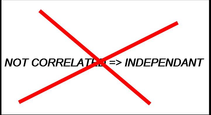
               variables are statistically linked together                                                variables are statistically independant



                     there is no correlation
               BUT variables are statistically linked together !


INDEPENDANT => NOT CORRELATED, and more important to keep in mind :




2 - cause to effect relation
Please DO NOT interpret correlation as cause to effect relation !
Indeed, for instantanous cause to effect relations, several different cause to effect schemes may lead to correlated variables : example
    . U -> V
   (V is a consequence of U)
    . W -> U
      &
      W -> V
  (U and V and 2 effects of the same cause : they may often vary together ... but there is no cause to effect relation between them : if you act on
  U, then it won't have any effect on V) : example : someone falls and then breack his/her arm and his/her leg ... do you think that fixing
  the arm will fix the leg ? If not, then it means there is no cause to effect relation between those 2 facts ...

Observation of variations on the very short term ALWAYS leads to a high correlation :

The 2 variations are not correlated (correlation = -0,2).
Now let us zoom in :


In the very short term, it often happens that 2 variations are highly correlated : here : correlation = 1.

There are many fields of applications where time contants of evolutions are very big (example : hundreds of thoursand years), while our observations are made on the very short term (a few years, or one hundred years ...). Estimations of correlations on such a kind of variations always lead to ... nonsense (but scientifically plausible nonsense !).

There are many bad uses of correlation even in "scientific" publications (ex : epidemiology applications).
Example : average life duration of people still grows in Europe; number of motors increases in Europe
It means that THERE IS A STRONG CORRELATION (close to "1") between those two variables ! Why not making a linear model adjusted to predict life duration from the number of motors ... (try it, it's easy, numbers are available on the internet ... you will get a model with a very good accuracy on last 30 years ... and every statistical test will tell you that relation is significant !) ... And using this model, please estimate how many motors are needed in order to let us live 1000 years ... (sounds silly ? ... well now think about it and read every paper that involve correlation and linear regression with that silly example in mind ...). In our example, one can understand that those 2 variables (increasing life duration, and increasing number of motors) are both the consequences of the same cause : progress (technical progress - medicine, engineering, ... - social progress - easy access to medicine, no need to be a millionaire to buy a car, ... - )

In addtition, one knows that cause to effect relations ARE NOT INSTANTANOUS (effects should come AFTER causes ...). Even in a linear relation hypothesis, then effect is obtained through the filtering of cause by an impulse response function that may lead to a null correlation between cause and effect ... Even after delaying one variable (because if h(t) ≠ d(t-i), then it not possible to recover the correlation just by a delay ... for more information please read SIGNAL THEORY) ... And be aware that most of the time, relations ARE not linear because the positive effects and the negative effects do not have the same inertia : example : you put lachrymatory gas in a room : a few seconds after, everyone in the room will have tears in the eye; now put off the gas ... it will take a few minutes to these persons to recover a dry eye ! ...
(you might have guessed now that epidemiology studies (for instance) ... need more know-how than just pushing the buttons of a cool stats software ... :-)

2 - scalar product between variables
One can demonstrate that variables may be considered as vectors, and correlation is then the scalar product. It means that interpretation may be the cosinus of the angle between those 2 vectors..
But cosinus is not linear ... and one can understand then that moving from 0,95 to 0,96 is not the same than moving from 0,11 to 0,12 ...
(although it is LINEAR correlation ... it's interpretation is NOT LINEAR).
Because the frontier that shares correlated vectors (close to 0 degree) from not correlated vectors (close to 90 degrees) is ... 45 degrees ... Then one cannot really say that correlation is strong beneath r = 0,707.

NB : the square of the correlation r, is called the coefficient of determination r². This estimator varies from 0 to 1. It's threshold of strongness is 0,5  (0,707²), but beware, r² varies fast between 0 and 0,5 and is quasi linear between 0,5 and 1 : it's interpretation is then as non linear as the interpretation of correlation :

On the above diagram, angular fitness is the normalized variation of angle to 90 degrees. One can see that the slope of angular fitness increases very fast when tending to 1, although for both estimators (r² and angular fitness) a correlation of 0,707 corresponds to an estimator value of 0,5.


Comparison of a quantitative variable and a qualitative one : F (Fisher Snedecor)

The problem now it to test if a qualitative variable (example : motor technology for a car) and a quantitative one (example : maximum speed for a car) are independant. These two variables are different characteristics of a same population (example : "cars"). The qualitative variable divides the population in several groups (example : old diesel, direct injection diesel, gazoline, blend electric/gazoline, ...). The quantitative variable is summarized by its mean and its standard deviation (one assumes that this way of summarizing makes sense : Gaussian distribution).
The variables are independant (null hypothesis) if the mean and the variance are the same in all the groups. The Fisher Snedecor test is made to compare the mean value equality. There is a test based on the Khi-2 to compare the variances. We consider now that the variances are equal in each group.
We calculate the variances :

   the global variance

     the inter class variance or variance of the means.

 the intra class variance or the mean of the variances

The F Test is : 

After we use tables of Fisher Snedecor to read the Theoretical F value at the row (n-k) and the column (k-1).

If Fcalc > F then the “null hypothesis” is rejected or in other words the two variables are dependant with a risk ratio to made a mistake. There is several tables for each risk ratio.

Comparison of two qualitative variables : Khi-2 (or Chi-2)

On of the most common methods to proof a correspondence between empirical data and an expected distribution is the Chi² test. This test gives an indication if the data fits the model. The test value can be calculated by

where :

n = number of possible different observations (elementary events or classes)

X_i = observed number of event i

E_i = (theoretical) expected number of event i.

Depending on the value of Chi² one can accept or reject the hypothesis that the theoretical model fits the data well. Tables for the critical values depending on a level of significance and the number of degrees of freedom (n-1) for the model can be found in any book about likelihood methods.

We use the Chi-2 to test if two qualitative variables are dependant or not. The “null hypothesis” or the variables are independent if the contingency table is equi-distributed.

For instance for this contingency array:

	x	y	total
a	4	1	5
b	2	11	13
Total	6	12	18

 

The equi-distributed array is :

	x	y	total
a	2	3	5
b	4	9	13
Total	6	12	18

Each cell Y(i,j) of this array with M rows and N columns is calculated from the contingency array X(i,j) with the formula :

The chi2  is calculated as :

The degrees of freedom for this test is (MN – 1).

When the hypothesis is verified (here : equirepartition), then Chi-2 = 0. The more the Chi-2 is high the more the tested hypothesis is faulse.
NB : equirepartition means "randomly" => no statistical link between the 2 qualitative variables. So one can say that Chi-2 is there a measure of statistical link between two qualitative variables.

---