In the 1940s, many searchers were involved into cybernetic researches. Their goal was to build artificial intelligent machines. Maintream research was logical modeling, knowledge representation, and knowledge based systems. These researches led many years further to expert systems, frames and objects, ...
A small number of searchers were following another way : they considered that the "best" intelligent "machine" was the human brain itself : this brain is supposed to be made of elementary cells (called neurons) highly connected together. "If one understand what this elementary cell does and how cells are connected together, then it should be possible to build artificial brains, and then to get intelligent machines". This mechanist view of intelligence led to research on biological neurons that were found to be an "electric component".
Unfortunately, it was also found that this elementary cell has got a strongly non linear behaviour. Well, non linear systems can be shared into two categories :
 - separable non linear systems : dynamic behaviour is ruled by a linear dynamic system, and a static non linear characteristic rules amplitude modifications,
 - non separable non linear systems : non linear characteristic of the system varies among time, and it is not possible to consider it as two separated subsystems : a linear dynamic one, and a static non linear one,
There exists maths theories that allow to predict the collective behaviour of a very big number of simple cells connected together (automata theory). There also exists maths theories that allow to predict the collective behaviour of a very small number of separable non linear cells poorly connected together (ex : first harmonic method, phase space method, ..., developped for non linear control applications, for oscillators engineering, ...).
Unfortunately, one doesn't have any theory that would allow to predict the collective behaviour of a very large number of non separable non linear cells highly connected together (connections are made through synapses that may amplify or inhibate the influence of inputs ... It is even possible to show that this behaviour might be strictly unpredictable (chaos theory) in much cases.
But biological neurons were found to have a non linear behaviour : under a certain threshold, inputs have no influence on output. They also were found to be non separable : ex : threshold value varies among time ... and last but not least ... neurons are connected to millions of their neighbours following very complex connection diagrams ...
That is why searchers Mac Culloch and Pitts decided to simplify their observations and built an "artificial neuron" also called "Mac Culloch and Pitts neuron".

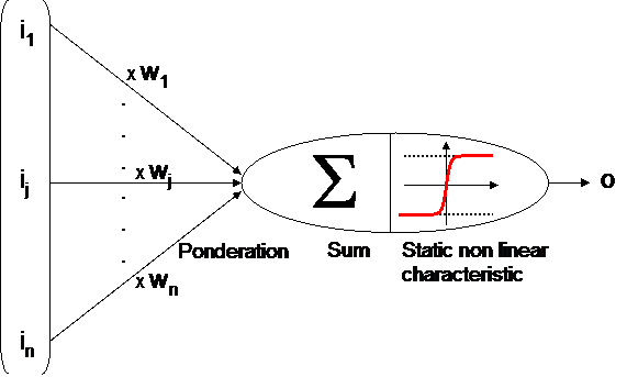
Coefficients w_j are called "synaptic weights". This elementary cell is still the one used nowadays in artificial neural networks applications.
One can notice that just before the non linear function (called activation function) the ponderation of the input vector by synaptic weights is the scalar product of input vector and synaptic weights vector :

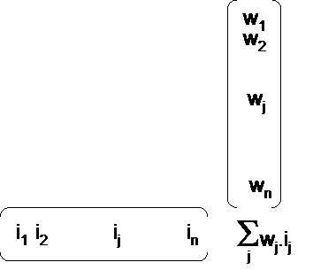
This scalar product is the left part of a hyperplan equation : Sw_j.i_j = 0
So one can see that if the w_j coefficients are tunable, then one have a tunable hyperplan (slopes, ...) that can be used for cutting space into 2 parts (classification) or for adjusting a set of data (regression).

---

From neurons to neural nets
There exist two main categories of neural networks :
 - feedback networks
 - feedforward multilayered networks
                             
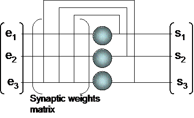
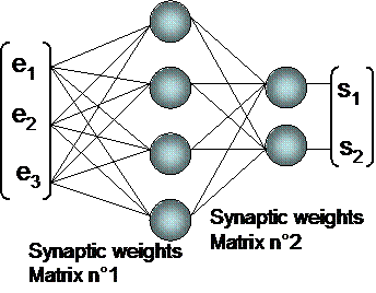
                    Feedback neural network                                                           Feedforward neural network

Feedforward multi layered neural networks can be considered as looped networks ... but with all feedback loops tuned at null synaptic weights. It means that feedback neural nets are the general case. Feedforward neural networks are a particular case. Inheritance gives them all properties of feedback networks ... but they also have particular properties :
 - always stable,
 - one could demonstrate that they are universal approximators,
Universal approximators are systems that can approximate functions, whatever complex the shape of this function may be ...
Their first layer is called "hidden layer".
Feedforward multilayered neural nets are the most applied in real world application, especially for modeling and pattern recognition applications.

---

Supervised learning

 - phase 3 : run the neural network,The principle of supervised learning can be described in 3 phases :
 - phase 1 : run of the network, on one or several input vectors,
 - phase 2 : compare the computed output with desired output on every example, and tune the neural net parameters in order to minimize the error,
 - phase 3 : run the neural network,


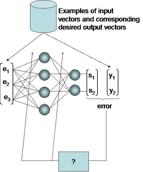
For a given neural network (number of neurons, ...), the only parameters to tune are the synaptic weights. The box "?" on the above diagram is supposed to tune the weights in order to minimize the output error. one call such a procedure a "learning rule".
One can consider error as a function of synaptic weights values :

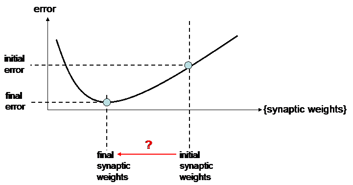
The random values of initial synaptic weights generally lead to a big error. So learning is finding a proper value for the synaptic weights, in order to find the minimum value for output error.

There are 2 main categories of supervised learning rules :
 - deteministic rules
 - random based rules

Deterministic learning rules
If you're "up" and wish to go "down" ... then follow the slopes ...
But slopes in every direction are given by the GRADIENT of error (on synaptic weights).
So the learning rule consists in computing the gradient among every synaptic weight of the neural network, and then modifying the weights in the gradient direction
This approach is not a neural network special one and you will find many references using keywords "optimization", and "operational research". Application of gradient method to neural networks is known as "backpropagation learning rule".
Main problems of such a learning rule comes froms local manima :

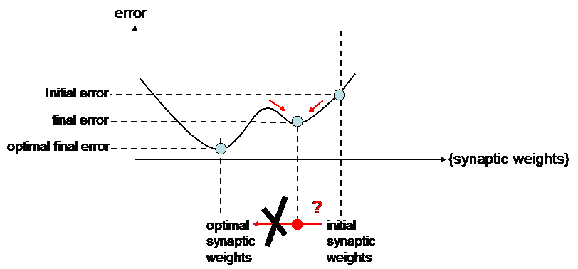
Indeed, following the slopes cannot always allow to get the optimal solution  : the modifications of synaptic weights may be trapped by local minima.
Several heuristics were imagined to avoird this local minima effect :
 - momentum,
 - stochastic/Widrow Hoff gradient,

Momentum :
The idea is to add inertia effect to synaptic weights modification : a low pass filter is applied to synaptic weights modifications : example : D W_ij applied = 0,5. D Wij given by gradient method + 0,5 . D W_ij applied at previous iteration
This inertia effect lets the modification run in the same direction for a few iterations even if the gradient changes of sign :

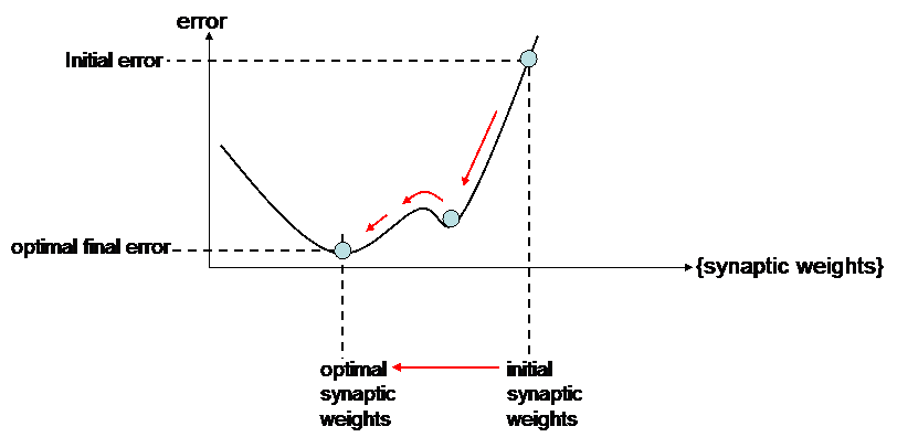
But oscillation will also happen when arriving at the optimal value (convergence will take more time).

Stochastic learning :
Instead of computing the error on every example, then adding all the errors and minimizing this global error, the idea is now to compute the output for 1 example, compute the error, and minimize it ... and then to do the same for the next example. One can understand that optimazing for a given example might de-optimize for another example ... However, one can demonstrate that in that case the learning rule should follow the slopes, but not strictly (not at every). This stochastic gradient may avoid to stay trapped in local minima.

But these methods are just heuristics : no demonstration of convergence to the right minima is available.

Random based learning rules
Sometimes following the slopes is not a good idea :

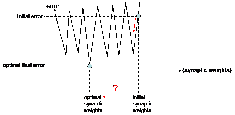
In such a case, only random filtering can be used for finding the optimal synaptic weights.
The 2 main methods then are :
 - random search
 - simulated annealing

random search :
This learning rule is :
 - try a modification of synaptic weights
 - if this modification leads to a better result (decreasing of global error), then keep it, else don't keep it
This rule is more "clever" than it seems. Indeed, all the idea is contained in the term "modification". Modification means that one goes to the new synaptic vector from the current synaptic vector by choosing a solution into a hypersphere centered at current position :

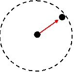
If we magnify the error function, one can see that ifever the hypersphere is very small, then the modifications still follow slopes (like a gradient method) :

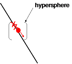
All modifications that lead to bigger errors are forgotten, and in the end the modification of weights follows the slopes of error function => this learning rule might be trapped by local minima !
In order to avoid being trapped, one can take a bigger hypersphere ... But if too big, then there is no sense anymore in the search : it might become "trying to find the right solution by chance" :

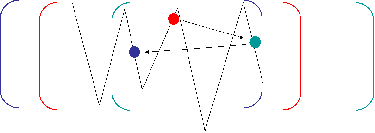
The difficulty of finding the "right" size of research hypersphere led to define a new heuristical method : the simulated annealing.

Simulated annealing :
This learning rule is :
 - try a modification of synaptic weights
 - if this modification leads to a better result (decreasing of global error), then keep it, else still keep it ... but with a certain probability (< 1)
At first iterations, probability to keep bad solutions is tuned at a rather hight level, and the more the iterations, the smallest the probability to keep bad solutions ...
Simulated annealing allows to avoid local minima even with a small size of hypersphere.

NB : supervised learning performance depends also to the quality of the learning examples :
 - complexity of the input output relation (preprocessings are often used in order to simplify this relation)
 - quality and number of examples : one must be sure that examples are a "good represention" of the reality,
 - generalization ability : test examples are often used in order to control that the neural network didn't learned "by heart" the learning data base.
All these elements can be tuned with the help of an engineering methodology built by NEXYAD main founders in the 1990s ("AGENDA methodology").

---

Unsupervised learning

Unsupervised learning in neural networks allows to build automatic clustering applications (like classical methods such as k-means). The idea is to minimize the error between inputs and ... synaptic weights. Then synaptic weights become an internal representation of inputs.


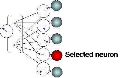
The neuron that is the closest to an input (*) is the selected neuron.
(*) distance between the input vector and every synaptic vector is computed. The neuron that corresponds to the smallest error is the selected neuron.
The selected neuron modifies its synaptic weights in order to minimize the error with the input (such a rule where only the selected neuron adjusts its weights is called "winner takes all" rule). Those who know classical data analysis methods should notice that such a neural network is just a stochastic implementation of the k-means algorithm.

In some learning rules (called "winner take most rules") the selected neuron also adjusts synaptic weights of its closest neighbourgs in the same direction.
There are two ways of estimating which neurons are the closest neighbourgs :

 - neighbourgs on a geographic map : then the neural net is called "self organization maps" (or Kohonen maps)
 - neighbourgs in the space of synaptic weights : the closest neighbourg of selected neuron A is the neuron that would have been selected in the place of A is A wouldn't exist. : then the neural nets is called "neural gas".

At the end of the learning process, one neuron is sensitive to one "kind" of inputs, called "class". In the case of self organization maps, then close neurons are sensitive to close classes (one says the network builds a topology in classes).

---

From neural nets to applications

Most applications shonw in papers and books can be decomposed on the basis of those 3 elementary applications :

- Automatic clustering :
     - neural nets methods : self organization maps, neural gas
     - alternative methods : k-means

 - Regression (modeling from a set of data) :
     - neural nets methods : feedforward neural nets and supervised learning
     - alternative methods : linear regressions

 - Classicifation / pattern recognition :
      - neural nets methods : feedforward neural nets and supervised learning
     - alternative methods : discriminant analysis, bayesian networks