

What is a
mathematical model ?
Keywords : mathematical model, what is a mathematical model, sensors, observing real world, observation of variations, experiment, sensors, measurement tools, finite range and precision sensors, functional analysis, modeling sub systems, global model, robust model,error of the model, prediction, forecasting, understanding, interpretation of parameters values,
Written by Gerard YAHIAOUI and Pierre DA SILVA DIAS, main founders of the applied maths research company NEXYAD, © NEXYAD, all rights reserved : for any question, please CONTACT
Reproduction of partial or complete content of this page is authorized ONLY if "source : NEXYAD http://www.nexyad.com" is clearly mentionned.
This tutorial was written for students or engineers that wish to get a synthetic view of what is called a "mathematical model". In particular, the intervention of human beings a priori ideas is very important and never explained in classical books that tend to prensent applied maths techniques as pure maths.
Definition : a mathematical model is not reality / a mathematical model is not pure maths
WHAT A MATHEMATICAL MODEL IS NOT
Mathematics may be defined as construction game leading to a big set of self-coherent intellectual entities : they do not have any existance outside of our head (no herd of "Twos" in the woods). This pure intellectual construction is mainly made by strange humans (called mathematicians) with no care of applications (except some exceptions). From this intellectual construction, other people (unbelievable but true) pick some maths entities and a priori decide to match them with some real world observations. These strange kind of people are called physicians, chemists, ... and applied maths engineers.
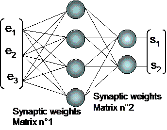
We show in the next figure the conceptual links between several maths-based human activities that lead together to what is generaly called a 'mathematical model' :
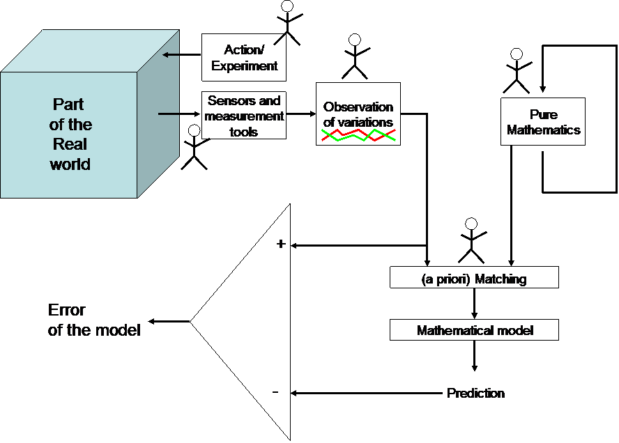
NB : Human being is the key element of main items in this scheme :
- Observing a part of the Real World through a finite number of sensors with finite resolution and range is a human activity : what to observe, using which sensors, why, ... are questions that find answers in a priori knowledge and belief of humans. For 'the same Real World', the choice of different experiments and sensors may lead to different observations (and then to different mathematics/observations matching).
- Building mathematics as a self coherent set of entities (what we could call 'pure maths'), discussing about what "self coherent" means, about what "demonstrated", or "exist" means, ... is a human intellectual activivity : ex : is it possible to create ex nihilo an entirely coherent system without a priori ? ... is a question that led to define the "axiom" notion (cf. the axiom of choice) that is the mathematical word for a priori knowledge and belief.
- Choosing to fit observations into pure maths entities, and then use inheritance of their properties and their ability to combine in order to build new entities, is a human activity using a priori knowledge and belief : ex : 'space' and 'time' are not fit into the same mathematical entities in Newton or in Einstein Physics ... does that mean that 'space' and 'time' properties have changed between 1665 and 1920 ? One can notice that experiments and observations techniques made big progress between those two dates ! and getting new observations of variations gave new 'ideas' of matching ... and led to new mathematical models.
Once every human activity has been done, then, we get MATHEMATICAL MODELS that are usually described in Universities as entirely self-coherent disciplines with no human intervention (and that is true : human intervention was to create them. Once model created, then inheritance allows to talk about observed entities with a vocabulary derived from pure maths, using formal combination operations ...). But it is important not to forget that :
- observations of variations ARE NOT the real world
- models ARE NOT the real world AT ALL
- models ARE NOT pure maths
Some facts that show their difference :
- observations give a representation of the real world, compatible with our senses (and mainly vision : we are can handle a 1, 2, or 3 D representation of an observation, not more !) in a finite range of precision, bandwith, ..., outside of this range, no one "knows" what's going on.
- mathematical models INTRINSICALLY produce ERRORS (of prediction/estimation ...) : once error is lower than a given value, one can say
that the MODEL IS "TRUE" (a very different definition of truth than in the pure maths world !).
NB : EVEN if the error seems to be null ... one should NEVER consider that the model is "perfect" because :
- measurements have a finite precision (so what a "null error" means ?)
- in practice, there always stays "small" unexplained variations called "noise"
- comparison between prediction of the model and observations was made ONLY in a finite number of cases
- experiment modifies the part of the real world that one tries to "observe" ... Observed variations are images of interactions between human beings and the "part of the world" ...
NB : the above diagram also shows that technology evolutions may lead to theoretical evolutions, although it is the opposite that is always presented as a feedforward cause to effect link in Universities ! (theoretical work is supposed to bring technology evolution).
WHAT A MATHEMATICAL MODEL IS
One could say that mathematical models (also called "applied maths" models) are nothing more than an intellectuel representation of a set of observations.
This intellectual representation has :
- finite range of application
- finite precision (error IS a characteristic of the representation)
And the representation may change :
- from a range of application to another,
- in time (nothing lasts forever ...),
WHAT THE HELL CAN I DO WITH SUCH A MATHEMATICAL MODEL ?
There are 2 main ways of using mathematical models :
1 - assuming that error is "small enough" to be considered as null :
In such a case, models are generally used for :
- forecasting : it is the first aim of a mathematical model : if i throw my arrow like this ... will it hit the animal ? If i construct this machine like that ... will it allow to do this ? ...
- "understanding" : if a model has "parameters" that may be tuned in order to adapt its output to observations (it means in order to get a quasi-null error on a set of observations), then sometimes, the parameters values are used as "descriptors" of the real world. For that, these parameters must have an intrinsic meaning for the human being that applies the model. NB : "understanding" the real world IS NOT possible through the use of applied maths, as shown on the above diagram ... one can only understand the "state" of our intellectual representation of the real world !
2 - hypothesis tester : detection and classification
In such a case, the error is not supposed as a quasi-null value : error is an image of the "distance" between the real world and our intellectual representation of the real world. Then this approach is often used in "detection" applications (defects detection, rare facts detection, ...), or classification (running several models in the same time allows to get several errors, each error corresponding to a given hypothesis; the smallest error corresponds to the most plausible known hypothesis).
AND IF MY SYSTEM IS COMPOSED OF MANY SUB-SYSTEMS ?
When the part of the real world (also called "system") is "big" (example : a car), temptation is to cut it into sub-systems (example : wheels, tires, springs, suspension, ...) and to build a model for every of them. This is the most seen option in the industry.
Unfortunately, this way of building applied maths models has 2 disadvantages :
- errors (of sub-models) may cumulate ... (and believe us ... they often do !), and in the end, the most detailed the model, the less usefull !
- the cutting of a system into sub-systems is often technology sensitive : example for a car : the mecanical steer can be decomposed into a few mecanical bodies ... But in case of a steer by wire (electronic steer), it is nonsense to keep the same decomposition (electronic sub systems don't mimic the functionalities of mecanical bodies of the mecanical steer).
It means the a FUNCTIONAL ANALYSIS must be done BEFORE building the model : subsystems must not be seenable bodies, they must be "sub-functions" (that are not supposed to be technology sensitive).
And in practice ... "global imprecise models" often lead to better results than detailed precise ones (because the more a sub-model is precise, the more it is sensitive to the error generated by the upstream sub-model ...).
In any case, one can see that precision of upstream sub models MUST be much better that precision of downstream sub models ... in order to get a robust model. If this is not the case, it is not possible to plug models on models ... without building a model of the interface (dealing with precision matters) : a model of the connexion between two models ... (stop !)
CAN I BUILD A MODEL FOR "ANYTHING" ?
The answer is NO.
Lets us consider the billboard game :
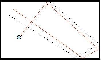
The black line is the desired trajectory. The red one is the real trajectory : angle and speed cannot be initialized with an infinite precision. This is called the error on initial conditions. One can see on the above diagram that this initial error grows in a regular way with time : for "every" time, it is possible to know in wich range the error is. One says that such a system can be modelized.
Now, let us consider exactly the same game, but with obstacles :
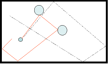
One can see that even for a very small initial error, trajectories may be completely different after a certain time : at the beginning, the system is predictable ... but suddenly a BIFURCATION occurs and the error goes out of bounds.
This sensitivity to initial conditions leads to the definition of chaotic systems : when sensitivity to initial conditions is bigger than precision of actuators and measurements ... the system is theoretically unpredictable in the long term (although it stays completely predictable in the short term !).
Building a model of the bilboard with obstacles wouldn't allow to get long term forecasting !
Several kinds of models
The God Knowledge Model
The first interesting model to describe is also the simplest to explain (although it is impossible to apply in practice) : this is the "God Knowledge Model" (GKM). This model is nothing else than a giant (infinite) data base with ALL the possible cases recorded.
In order to get the output of the model, one needs the input vector : this input vector has to be found into the data base.
Once found, one only has to READ the output.
There is no computing.
Of course, the number of cases is generally infinite (and even not countable) and this model cannot be used ... But let's keep it in mind !
Characteristics : infinite number of data points, no computing.
The Local Computing Memory
The idea that comes next to the GOD KNOWLEDGE model is the LOCAL COMPUTING MEMORY : this solution consists in recording "almost every possible observation" into a big data base. Then when a partial observation occurs, it is possible to search for the closest record in this data base (let's notice that this notion of closeness between sets of measures request that a topology and then a distance have to be defined before).
When the 2 or 3 closest cases are found, then it is possible to COMPUTE the output of the new entry (ex : a vote procedure for a pattern recognition/classification system, an interpolation/extrapolation procedure for a quantitative modeling system).
One can see that it is possible to consider the God Knowledge Model as a limit of the Local Computing Memory when the number of recorded cases tends to ALL THE CASES.
Computings are a local procedure (it applies only between the few elements selected because they are very "close" to the new entry).
Characteristics : low computing power, big memory.
The Equational Model
The equational model is a set of mathematical equations : example :
y = ax2 + bx + c ; in this example, y can be considered as an output variable, x as an input variable, and a, b, c as parameters.
The equations are usually given by a "theory" (a set of a priori matching between observations and maths entities that were shown to be interesting and that is tought, for instance, in universities) or they may result from YOUR experiments. The parameters have to be tuned in order to make predictions fit into measurements : one must find a "good set of parameters". In the general case, there is no UNIQUE set of parameters for a given result.
There are mainly two ways of finding such a parameters set :
- a priori : parameters must have then an intrinsic meaning for an expert that uses a theory involving these parameters (physics, ...),
- from data : parameters are automatically tuned in order to maximize the fitness of the model (compared to real data) : maximizing the fitness usually means minimizing the error of the model.
This second way of finding a good set of parameters doesn't need them to have an "intrinsic meaning". The search for a good set of parameters that will lead the model to fit into observations is often called "process identification".
NB : there may be several equational systems for several ranges of variation (plus a switch). Ifever "every" case needs a new set of equations, then it means that equations are not needed : one just need to record the output for a given input, and the system becomes a God Knowledge System. On the opposite, if ONE system of equations can be used, whatever input range, then one call it a General Equational Model. In the case of understandable parameters, the model is said to be a "knowledge based general equational model".
Characteristics : high computing power, low memory.
NB : because model and parameters are chosen in order to make prediction fit into observations on a FINITE set of examples, the General Equational Model doesn't exist in practice (it has LIMITS OF APPLICABILITY). It is very important that the user is aware of these limits ...
Equational models that show a "meaning" through their parameters
Example : U = U0.e-t/t
Parameters are U0 and t.
Input is t.
Output is U.
Meaning of parameters : U0 is the initial value, and t is the inertia (intersection between U = 0 and the trend with slope for t = 0) :
Equational models that show a meaning through their parameters are often called "white boxes".
Equational models that show "no meaning" through their parameters
Example 1 : the so-called feed forward Neural Networks (see NEURAL NETS)
Let us consider M1 = synaptic weights matrix n°1, M2 = synaptic weights matrix n°2, then :
Si = th(SM2ij.(th(SM1jk.ek)) )
This kind of equations, under certain conditions, are universal approximators (see HERE), and they are used for modeling systems from data. Parameters are the synaptic weights (values of matrix 1 and matrix 2) and they generally do not have any intrinsic meaning for the user of such a model. That is why they are often called "black boxes".
Example 2 : sometimes, even very simple equational model don't show any meaning through their parameters
Let us consider the linear regression model : Y = SaiXi + error
The parameters are the ai coefficients. They are computed by the linear regression algorithm in order to fit the model into observations.
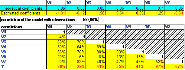
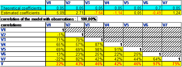
Because the model is very simple, coefficients are supposed to have a meaning for the user ... (ex : a kind of "weight" or "importance" ...), but we show below an example (Excel simulation : everyone can try on his/her computer) :
- We build a set of data :
V1 = alea(); V2 = 0,1.V1 + ALEA(); V3 = 0,5.V1 + 0,5.V2; V4 = 0,3.V3 + 0,3.V2 + 0,3.V1 - ALEA()/3;
V5 = ALEA()/10 + 0,25.V4+0,25.V3+0,25.V2+0,25.V1; V6 = ALEA()-0,1.V1 - 0,2.V2 + 0,6.V5; V7 = V6+V5+V2 - V1
And Y = 0,05.V1 + 0,05.V2 + 0,05.V3 + 0,05.V4 + 0,05.V5 + 0,7.V6 + 0,05.V7
- Every time that we click the F9 key, new random values ALEA() are given, and the linear regression algorithm of Excel is applied. This linear regression algorithms leads to two interesting set of results :
- the set of ai parameters of the model : this set of parameters can be compared to the parameters actually used to build Y.
- the correlation of reconstruction (expected : 100%) = fitness of the model
We give the correlation matrix for every F9 click, in order to let statisticians think about it :-)
results :
- click F9 n°1 :
- click F9 n°2 :
- etc ...
conclusion : Process identification with a linear regression always lead, in our case, to a "PERFECT" model (correlation = 1).
However, even if the model is "perfect" in terms of correlation ... and even if this model is very simple ... its parameters have NO meaning !
(although interpretation of regression coefficients as "importance measurement" is a method that many universities still apply and even publish in "scientifical" papers ... Unfortunately, this is not possible unless certain conditions of independance of input variables ... that are RARELY verified in practice !) : the "perfect theory applied to cases where it shouldn't apply ... leads to the "perfect publishable nonsense" !
The rules-based model
Sometimes, knowledge and belief about observed variations are not "recorded" neither as data nor as equations : indeed, they also can be recorded as a set of "rules" :
examples :
"if this happens, consequence will be xxxx"
"the more the pressure growing, the more the temperature growing, the less the volume ..."
Rules are a set of logical entities that describe the variations in a QUALITATIVE way (some say in a symbolic world).
In order to allow a quantitative evaluation of the "model's output", there are several approches : the most known are :
- case-based reasonning, that proposes to apply the closest recorded case (so one can see its closeness to local computing memories),
- Bayesian probabilties systems : knowing that A and B have a probability of P(A) and P(B), what is the probability P(C) for C ?
- fuzzy logic, that describes rules with numerical representation among quantitative variables (see FUZZY LOGIC), allows very easily to transform numerical data into concepts, apply logic on concepts entities, and convert back the conclusion of logical processing into a numerical result.
Advantage of rules-based systems is that their behaviour is understandable in natural language. Disadvantage is that rules are a less compact way of recording knowledge and belief than equations.
Characteristics : average computing power, average memory.
Conclusion
Building applied maths models is a work for experts ...
The use of a software's user friendly interface may produce many numbers and simulations that have no meaning at all ... although they bring the "illusion" of truth !
The main points are :
- focus on the "good" level of details (use a functional analysis ...),
- take into account the error of models as an intrinsic properties of applied maths models (if you wish to get robust models),
- choose an applicable kind of model (if you need data for process identification ... make sure that data are available ...),
- don't try to build a long term forecasting model for a chaotic system,
- verify in "reality" hypothesis of applicability ,
- give limits of the model validity domain (ranges ...), it will avoid eccentric extrapolations ! ...
- beware, if you try in give a meaning to parameters, it's not that simple : if equations come from a knowledge, then it might be possible, but even in such a case, one must verify a few conditions.
Keywords : mathematical model, what is a mathematical model, sensors, observing real world, observation of variations, experiment, sensors, measurement tools, finite range and precision sensors, functional analysis, modeling sub systems, global model, robust model,error of the model, prediction, forecasting, understanding, interpretation of parameters values,
Written by Gerard YAHIAOUI and Pierre DA SILVA DIAS, main founders of the applied maths research company NEXYAD, © NEXYAD, all rights reserved : for any question, please CONTACT
Reproduction of partial or complete content of this page is authorized ONLY if "source : NEXYAD http://www.nexyad.com" is clearly mentionned.
This tutorial was written for students or engineers that wish to get a synthetic view of what is called a "mathematical model". In particular, the intervention of human beings a priori ideas is very important and never explained in classical books that tend to prensent applied maths techniques as pure maths.
Definition : a mathematical model is not reality / a mathematical model is not pure maths
WHAT A MATHEMATICAL MODEL IS NOT
Mathematics may be defined as construction game leading to a big set of self-coherent intellectual entities : they do not have any existance outside of our head (no herd of "Twos" in the woods). This pure intellectual construction is mainly made by strange humans (called mathematicians) with no care of applications (except some exceptions). From this intellectual construction, other people (unbelievable but true) pick some maths entities and a priori decide to match them with some real world observations. These strange kind of people are called physicians, chemists, ... and applied maths engineers.
We show in the next figure the conceptual links between several maths-based human activities that lead together to what is generaly called a 'mathematical model' :
NB : Human being is the key element of main items in this scheme :
- Observing a part of the Real World through a finite number of sensors with finite resolution and range is a human activity : what to observe, using which sensors, why, ... are questions that find answers in a priori knowledge and belief of humans. For 'the same Real World', the choice of different experiments and sensors may lead to different observations (and then to different mathematics/observations matching).
- Building mathematics as a self coherent set of entities (what we could call 'pure maths'), discussing about what "self coherent" means, about what "demonstrated", or "exist" means, ... is a human intellectual activivity : ex : is it possible to create ex nihilo an entirely coherent system without a priori ? ... is a question that led to define the "axiom" notion (cf. the axiom of choice) that is the mathematical word for a priori knowledge and belief.
- Choosing to fit observations into pure maths entities, and then use inheritance of their properties and their ability to combine in order to build new entities, is a human activity using a priori knowledge and belief : ex : 'space' and 'time' are not fit into the same mathematical entities in Newton or in Einstein Physics ... does that mean that 'space' and 'time' properties have changed between 1665 and 1920 ? One can notice that experiments and observations techniques made big progress between those two dates ! and getting new observations of variations gave new 'ideas' of matching ... and led to new mathematical models.
Once every human activity has been done, then, we get MATHEMATICAL MODELS that are usually described in Universities as entirely self-coherent disciplines with no human intervention (and that is true : human intervention was to create them. Once model created, then inheritance allows to talk about observed entities with a vocabulary derived from pure maths, using formal combination operations ...). But it is important not to forget that :
- observations of variations ARE NOT the real world
- models ARE NOT the real world AT ALL
- models ARE NOT pure maths
Some facts that show their difference :
- observations give a representation of the real world, compatible with our senses (and mainly vision : we are can handle a 1, 2, or 3 D representation of an observation, not more !) in a finite range of precision, bandwith, ..., outside of this range, no one "knows" what's going on.
- mathematical models INTRINSICALLY produce ERRORS (of prediction/estimation ...) : once error is lower than a given value, one can say
that the MODEL IS "TRUE" (a very different definition of truth than in the pure maths world !).
NB : EVEN if the error seems to be null ... one should NEVER consider that the model is "perfect" because :
- measurements have a finite precision (so what a "null error" means ?)
- in practice, there always stays "small" unexplained variations called "noise"
- comparison between prediction of the model and observations was made ONLY in a finite number of cases
- experiment modifies the part of the real world that one tries to "observe" ... Observed variations are images of interactions between human beings and the "part of the world" ...
NB : the above diagram also shows that technology evolutions may lead to theoretical evolutions, although it is the opposite that is always presented as a feedforward cause to effect link in Universities ! (theoretical work is supposed to bring technology evolution).
WHAT A MATHEMATICAL MODEL IS
One could say that mathematical models (also called "applied maths" models) are nothing more than an intellectuel representation of a set of observations.
This intellectual representation has :
- finite range of application
- finite precision (error IS a characteristic of the representation)
And the representation may change :
- from a range of application to another,
- in time (nothing lasts forever ...),
WHAT THE HELL CAN I DO WITH SUCH A MATHEMATICAL MODEL ?
There are 2 main ways of using mathematical models :
1 - assuming that error is "small enough" to be considered as null :
In such a case, models are generally used for :
- forecasting : it is the first aim of a mathematical model : if i throw my arrow like this ... will it hit the animal ? If i construct this machine like that ... will it allow to do this ? ...
- "understanding" : if a model has "parameters" that may be tuned in order to adapt its output to observations (it means in order to get a quasi-null error on a set of observations), then sometimes, the parameters values are used as "descriptors" of the real world. For that, these parameters must have an intrinsic meaning for the human being that applies the model. NB : "understanding" the real world IS NOT possible through the use of applied maths, as shown on the above diagram ... one can only understand the "state" of our intellectual representation of the real world !
2 - hypothesis tester : detection and classification
In such a case, the error is not supposed as a quasi-null value : error is an image of the "distance" between the real world and our intellectual representation of the real world. Then this approach is often used in "detection" applications (defects detection, rare facts detection, ...), or classification (running several models in the same time allows to get several errors, each error corresponding to a given hypothesis; the smallest error corresponds to the most plausible known hypothesis).
AND IF MY SYSTEM IS COMPOSED OF MANY SUB-SYSTEMS ?
When the part of the real world (also called "system") is "big" (example : a car), temptation is to cut it into sub-systems (example : wheels, tires, springs, suspension, ...) and to build a model for every of them. This is the most seen option in the industry.
Unfortunately, this way of building applied maths models has 2 disadvantages :
- errors (of sub-models) may cumulate ... (and believe us ... they often do !), and in the end, the most detailed the model, the less usefull !
- the cutting of a system into sub-systems is often technology sensitive : example for a car : the mecanical steer can be decomposed into a few mecanical bodies ... But in case of a steer by wire (electronic steer), it is nonsense to keep the same decomposition (electronic sub systems don't mimic the functionalities of mecanical bodies of the mecanical steer).
It means the a FUNCTIONAL ANALYSIS must be done BEFORE building the model : subsystems must not be seenable bodies, they must be "sub-functions" (that are not supposed to be technology sensitive).
And in practice ... "global imprecise models" often lead to better results than detailed precise ones (because the more a sub-model is precise, the more it is sensitive to the error generated by the upstream sub-model ...).
In any case, one can see that precision of upstream sub models MUST be much better that precision of downstream sub models ... in order to get a robust model. If this is not the case, it is not possible to plug models on models ... without building a model of the interface (dealing with precision matters) : a model of the connexion between two models ... (stop !)
CAN I BUILD A MODEL FOR "ANYTHING" ?
The answer is NO.
Lets us consider the billboard game :
The black line is the desired trajectory. The red one is the real trajectory : angle and speed cannot be initialized with an infinite precision. This is called the error on initial conditions. One can see on the above diagram that this initial error grows in a regular way with time : for "every" time, it is possible to know in wich range the error is. One says that such a system can be modelized.
Now, let us consider exactly the same game, but with obstacles :
One can see that even for a very small initial error, trajectories may be completely different after a certain time : at the beginning, the system is predictable ... but suddenly a BIFURCATION occurs and the error goes out of bounds.
This sensitivity to initial conditions leads to the definition of chaotic systems : when sensitivity to initial conditions is bigger than precision of actuators and measurements ... the system is theoretically unpredictable in the long term (although it stays completely predictable in the short term !).
Building a model of the bilboard with obstacles wouldn't allow to get long term forecasting !
Several kinds of models
The God Knowledge Model
The first interesting model to describe is also the simplest to explain (although it is impossible to apply in practice) : this is the "God Knowledge Model" (GKM). This model is nothing else than a giant (infinite) data base with ALL the possible cases recorded.
In order to get the output of the model, one needs the input vector : this input vector has to be found into the data base.
Once found, one only has to READ the output.
There is no computing.
Of course, the number of cases is generally infinite (and even not countable) and this model cannot be used ... But let's keep it in mind !
Characteristics : infinite number of data points, no computing.
The Local Computing Memory
The idea that comes next to the GOD KNOWLEDGE model is the LOCAL COMPUTING MEMORY : this solution consists in recording "almost every possible observation" into a big data base. Then when a partial observation occurs, it is possible to search for the closest record in this data base (let's notice that this notion of closeness between sets of measures request that a topology and then a distance have to be defined before).
When the 2 or 3 closest cases are found, then it is possible to COMPUTE the output of the new entry (ex : a vote procedure for a pattern recognition/classification system, an interpolation/extrapolation procedure for a quantitative modeling system).
One can see that it is possible to consider the God Knowledge Model as a limit of the Local Computing Memory when the number of recorded cases tends to ALL THE CASES.
Computings are a local procedure (it applies only between the few elements selected because they are very "close" to the new entry).
Characteristics : low computing power, big memory.
The Equational Model
The equational model is a set of mathematical equations : example :
y = ax2 + bx + c ; in this example, y can be considered as an output variable, x as an input variable, and a, b, c as parameters.
The equations are usually given by a "theory" (a set of a priori matching between observations and maths entities that were shown to be interesting and that is tought, for instance, in universities) or they may result from YOUR experiments. The parameters have to be tuned in order to make predictions fit into measurements : one must find a "good set of parameters". In the general case, there is no UNIQUE set of parameters for a given result.
There are mainly two ways of finding such a parameters set :
- a priori : parameters must have then an intrinsic meaning for an expert that uses a theory involving these parameters (physics, ...),
- from data : parameters are automatically tuned in order to maximize the fitness of the model (compared to real data) : maximizing the fitness usually means minimizing the error of the model.
This second way of finding a good set of parameters doesn't need them to have an "intrinsic meaning". The search for a good set of parameters that will lead the model to fit into observations is often called "process identification".
NB : there may be several equational systems for several ranges of variation (plus a switch). Ifever "every" case needs a new set of equations, then it means that equations are not needed : one just need to record the output for a given input, and the system becomes a God Knowledge System. On the opposite, if ONE system of equations can be used, whatever input range, then one call it a General Equational Model. In the case of understandable parameters, the model is said to be a "knowledge based general equational model".
Characteristics : high computing power, low memory.
NB : because model and parameters are chosen in order to make prediction fit into observations on a FINITE set of examples, the General Equational Model doesn't exist in practice (it has LIMITS OF APPLICABILITY). It is very important that the user is aware of these limits ...
Equational models that show a "meaning" through their parameters
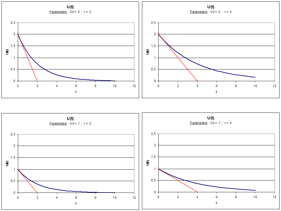
Example : U = U0.e-t/t
Parameters are U0 and t.
Input is t.
Output is U.
Meaning of parameters : U0 is the initial value, and t is the inertia (intersection between U = 0 and the trend with slope for t = 0) :
Equational models that show a meaning through their parameters are often called "white boxes".
Equational models that show "no meaning" through their parameters
Example 1 : the so-called feed forward Neural Networks (see NEURAL NETS)
Let us consider M1 = synaptic weights matrix n°1, M2 = synaptic weights matrix n°2, then :
Si = th(SM2ij.(th(SM1jk.ek)) )
This kind of equations, under certain conditions, are universal approximators (see HERE), and they are used for modeling systems from data. Parameters are the synaptic weights (values of matrix 1 and matrix 2) and they generally do not have any intrinsic meaning for the user of such a model. That is why they are often called "black boxes".
Example 2 : sometimes, even very simple equational model don't show any meaning through their parameters
Let us consider the linear regression model : Y = SaiXi + error
The parameters are the ai coefficients. They are computed by the linear regression algorithm in order to fit the model into observations.
Because the model is very simple, coefficients are supposed to have a meaning for the user ... (ex : a kind of "weight" or "importance" ...), but we show below an example (Excel simulation : everyone can try on his/her computer) :
- We build a set of data :
V1 = alea(); V2 = 0,1.V1 + ALEA(); V3 = 0,5.V1 + 0,5.V2; V4 = 0,3.V3 + 0,3.V2 + 0,3.V1 - ALEA()/3;
V5 = ALEA()/10 + 0,25.V4+0,25.V3+0,25.V2+0,25.V1; V6 = ALEA()-0,1.V1 - 0,2.V2 + 0,6.V5; V7 = V6+V5+V2 - V1
And Y = 0,05.V1 + 0,05.V2 + 0,05.V3 + 0,05.V4 + 0,05.V5 + 0,7.V6 + 0,05.V7
- Every time that we click the F9 key, new random values ALEA() are given, and the linear regression algorithm of Excel is applied. This linear regression algorithms leads to two interesting set of results :
- the set of ai parameters of the model : this set of parameters can be compared to the parameters actually used to build Y.
- the correlation of reconstruction (expected : 100%) = fitness of the model
We give the correlation matrix for every F9 click, in order to let statisticians think about it :-)
results :
- click F9 n°1 :
- click F9 n°2 :
- etc ...
conclusion : Process identification with a linear regression always lead, in our case, to a "PERFECT" model (correlation = 1).
However, even if the model is "perfect" in terms of correlation ... and even if this model is very simple ... its parameters have NO meaning !
(although interpretation of regression coefficients as "importance measurement" is a method that many universities still apply and even publish in "scientifical" papers ... Unfortunately, this is not possible unless certain conditions of independance of input variables ... that are RARELY verified in practice !) : the "perfect theory applied to cases where it shouldn't apply ... leads to the "perfect publishable nonsense" !
The rules-based model
Sometimes, knowledge and belief about observed variations are not "recorded" neither as data nor as equations : indeed, they also can be recorded as a set of "rules" :
examples :
"if this happens, consequence will be xxxx"
"the more the pressure growing, the more the temperature growing, the less the volume ..."
Rules are a set of logical entities that describe the variations in a QUALITATIVE way (some say in a symbolic world).
In order to allow a quantitative evaluation of the "model's output", there are several approches : the most known are :
- case-based reasonning, that proposes to apply the closest recorded case (so one can see its closeness to local computing memories),
- Bayesian probabilties systems : knowing that A and B have a probability of P(A) and P(B), what is the probability P(C) for C ?
- fuzzy logic, that describes rules with numerical representation among quantitative variables (see FUZZY LOGIC), allows very easily to transform numerical data into concepts, apply logic on concepts entities, and convert back the conclusion of logical processing into a numerical result.
Advantage of rules-based systems is that their behaviour is understandable in natural language. Disadvantage is that rules are a less compact way of recording knowledge and belief than equations.
Characteristics : average computing power, average memory.
Conclusion
Building applied maths models is a work for experts ...
The use of a software's user friendly interface may produce many numbers and simulations that have no meaning at all ... although they bring the "illusion" of truth !
The main points are :
- focus on the "good" level of details (use a functional analysis ...),
- take into account the error of models as an intrinsic properties of applied maths models (if you wish to get robust models),
- choose an applicable kind of model (if you need data for process identification ... make sure that data are available ...),
- don't try to build a long term forecasting model for a chaotic system,
- verify in "reality" hypothesis of applicability ,
- give limits of the model validity domain (ranges ...), it will avoid eccentric extrapolations ! ...
- beware, if you try in give a meaning to parameters, it's not that simple : if equations come from a knowledge, then it might be possible, but even in such a case, one must verify a few conditions.
For
more questions or applications,
please feel free to contact
us