

Virtual sensors :
tutorial
Keywords : tutorial, virtual sensor, estimation, observation, state vector, input vector, state model, observation model, inverse model, correction gain, linear systems, observability, observability condition, observation theory, asymptotic, stochastic, locked loop, belief, optimal filtering, measurement, noise, noise distribution, eigen values, eigen vectors, kalman, luenberger, nexyad, applied maths,
Written by Gerard YAHIAOUI and Pierre DA SILVA DIAS, main founders of the applied maths research company NEXYAD, © NEXYAD, all rights reserved : for any question, please CONTACT
Reproduction of partial or complete content of this page is authorized ONLY if "source : NEXYAD http://www.nexyad.com" is clearly mentionned.
This tutorial was written for students or engineers that wish to understand main hypothesis and ideas of virtual sensors.
Vocabulary and questions
Frequent
Asked Questions (FAQs)

FAQ 1 : if you know Model 1, why don't you simply use it to find S(t) ?
If you wish to simply use Model 1 in order to reconstruct S(t), then you need to know first U(t-k) AND S(t-1).
U(t-k) is known (inputs of the system), but concerning S(t-1), it's not that simple ! ...
(remind that you don't have a sensor for S => you cannot know S(t-1) ... ).
In some applications, it is possible to put the system in an "obvious" state (example : starting point for a car : before for unlock the parck brake : speed = 0, longitudinal acceleration = 0, ...). It means that in such a case, S(0) is known without needing sensors.
Then, application of Model 1 will lead succesively to S(1), S(2), ..., S(t-1), S(t), ...
NB : knowing S(t-1) and U(t-k), application of Model 1 is a feedforward process : the modeling error cumulates among iterations.
It means that the more the iterations, the less the precision of estimation.
FAQ 2 : if you know Model 2, why don't you simply inverse this model in order to build S(t) from Ym(t) ?
Ifever this is possible, then YES, you should inverse Model 2.
Generally, Model 2 is injective : one only measure a few consequences of S(t).
In such a case, there exists several inputs of Model 2 that lead to the same output value, and "more" equations are needed in order to choose the right input value.
Because S(t) is produced by Model 1 ... THIS IS THE ROLE OF Model 1 ! to give more equations that S(t) MUST fit into
Example : self coherence among time.
Condition is then to verify that supplementary equations given by Model 1 are independant on equations given by Model 2. When this condition is verified, one say that S(t) is "observable" through the virtual sensor (see below "observability").
A very simple "handmade" example

D = (c1.a11 + c2.a21 ) . (c2 ) - (c1 ) . (c1.a12 + c2.a22 ) ≠ 0
Under this condition, one can determinate s1(t-1) and s2(t-1)
Applying Model 1 to s1(t-1) and s2(t-1), one get s1(t) and s2(t).
Numerical example :


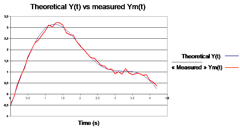
One builds a Y(t) signal, and we add some random noise in order to get a "measured" Ym(t).
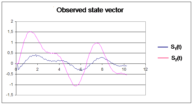
S1(t) and S2(t) are estimated, although one never measured them : this is called a virtual sensor of vector S.
The iterative locked loop estimation idea
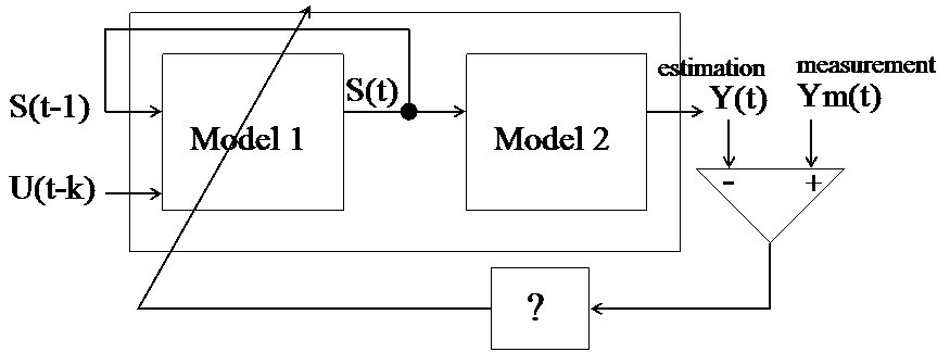
The idea is to compare Y(t) with Ym(t) and to "automatically adjust" Model 1 in order to minimize the error. Under conditions of "observability" (see below), one consider that X(t) is well estimated when error is very near zero.

In this diagram, the bloc "?" is the minimization of the output error. The locked loop allows to verify that estimated values of S(t) lead to the proper output Ym(t). If not, then it means that estimated S(t) should be modified.
Because S(t) is produced by Model 1, one can consider that a modification of S(t) is in fact a modification of Model 1.
The idea of "not copying noise"
The idea is to compare Y(t) with Ym(t) and to "automatically adjust" Model 1 in order to minimize the error. Ifever there is noise added with Ym(t), then minimizing the error will lead to "copy" the noise from Ym(t) to Y(t) ...
Then taking into account existence of noise (knowledge based approach) may lead to tolerate a residual error on Y(t).
General case of linear systems
Observability condition
State equation : X(t) = A.X(t-1) + B.U(t-p)
Observation equation : Y(t) = C.X(t)
A is a n x n matrix.
One can demonstrate that the system is observable if (and only if) the matrix :
(CT | AT.CT | (AT)2.CT | … | (AT)(n-1).CT)
is a rank n matrix.
NB : in special case when A is written in the Eigen vectors base, then A is a diagonal matrix, and condition of observability becomes more simple : C must not have a null column.
Interesting way of writing equations
State equation : S(t) = A.S(t-1) + B.U(t-p)
Observation equation : Y(t) = C.S(t)
S is the state vector
U is the input vector
Y is the output vector
Ŝi/j is the predicted value for vector S at time i from the knowledge of every signals at time j
Ŷi/j is the predicted value for vector Y at time i from the knowledge of every signals at time j
Diagram :

First phase, at time k, consists in applying the models for predicting S at time (k+1), knowing every signal at time k :
Ŝk+1/k = A.Ŝk/k + B.Uk-i and Ŷk+1/k = C.Ŝk+1/k
Diagram :

Second phase, at time (k+1), consists in computing the error between Ŷk+1/k and the measure Yk+1
Ỹk+1/k = Yk+1 - Ŷk+1/k
This error is a "knowledge" : one predicted the value of Yk+1Yk , and The idea is to make a correction of Ŝ in order to take into account the error Ỹk+1 that was produced by Ŝk+1/k
The correction is in proportion to the error, and leads to an estimation of S at time (k+1), knowing every other signals until time (t+1) :
Ŝk+1/k+1 = Ŝk+1/k + Lk+1 . Ỹk+1 (3)
L is called the correction gain.
Replacing Ỹk+1 by its expression into 3 leads to :
Ŝk+1/k+1 = Ŝk+1/k + Lk+1 . (Yk+1 - Ŷk+1/k)= A.Ŝk/k + B.BUk-i + Lk+1 . (Yk+1 - Ŷk+1/k)
Ŝk+1/k+1 = A.Ŝk/k + B.Uk-i + Lk+1 . (Yk+1 - C.Ŝk+1/k )
Ŝk+1/k+1 = A.Ŝk/k + B.Uk-i + Lk+1 . (Yk+1 - C.(A.Ŝk/k + B.Uk-i ) )
Ŝk+1/k+1 = (I - Lk+1.C).A.Ŝk/k + (I - Lk+1.C).B.Uk-i + Lk+1.Yk+1
Diagram :

There exists several methods to compute the correction gain Lk+1
(see below)
Third phase, still at time (t+1), consists in applying the corrected model
The complete diagram is then :

One uses to record the residual error : Ỹk+1/k+1 = Yk+1 - Ŷk+1/k+1
If one decide to keep the new state model for next step, then one can call the system an "adaptive" virtual sensor.
If not, one computes next "first phase" using initial model.
NB : this way of decomposing the linear estimation of S(t) into 3 phases :
- prediction leading to an error between measurement (that is considered as a desired output) and computed output
- model 1 modification (in order to minimize error between desired output and computed output)
- estimation (application of the model)
allows to make a link between linear virtual sensors theory and other applied maths techniques such as neural networks, for instance, that involve exactly the same 3 phases (cf. NEURAL NETS).
Estimation of a good correction gain L
Asymptotic methods :
Let us consider the error made on S estimation at time (k+1) :
Šk+1/k = Sk+1 - Ŝk+1/k+1
Šk+1/k = (A.Sk + B.Uk-i ) - ( (I - Lk+1.C).A.Ŝk/k + (I - Lk+1.C).B.Uk-i + Lk+1.Yk+1 )
Šk+1/k = (A.Sk + B.Uk-i ) - ( (I - Lk+1.C).A.Ŝk/k + (I - Lk+1.C).B.Uk-i + Lk+1.Yk+1 )
after some obvious manipulation, one get :
Šk+1/k = (I - Lk+1.C).A. Šk/k
This recurrence is asymptotic if the Eigen values of matrix (I - Lk+1.C).A have their module smaller than 1 ( such a matrix is called a Schur matrix ).
It means that there exists "many" methods to choose the correction gain.
Some famous methods are :
- Luenberger method : change of variable in order to get a canonical form of the system that leads to a simple way of choosing a gain Lk+1 S
- Minimization of a quadratic linear form
- ...
Stochastic methods :
This approach considers that models are not perfect. Their imperfection is considered as a random noise :
- a state model noise
- an observation model noise.
Every iteration, noise is amplified by the C matrix, and then Ŷk+1/k is corrupted with noise.
In such a case, it is obvious that the error (Yk+1 - Ŷk+1/k ) has not the same meaning : a null error means that one tries to copy the noise : if you try to estimate Y including noise of the models, then (because models are pure deterministic systems) the only solution is to add noise to S too ...
The idea of stochastic methods is to take into account imperfection of models and trying to go right in the middle of the noise distribution.
Intuitively, while output error is smaller than noise, then it is not necessary to apply a correction gain. This idea leads to other methods based on sets theory (not explained in this page) ... Stochastic approach should propose a model of noise and use it in order to minimize the influence of noise.
Estimation theory allows to write correction as the average value of prediction error :
Ŝk+1/k+1 = Ŝk+1/k + E{ Ŝk+1/k / Ŷk+1/k } (4) : mathematic belief of S, knowing the prediction of Y
(4) simply means that correction should be the average value of error made when Yk+1 is predicted with the value Ŷk+1/k
Comparison between (3) and (4) using conditional belief and probability density distribution leads to an iterative estimation of Lk+1 (but densities of noise probability has to be known).
Examples of applications
Simulating without cumulating noise among simulation duration :
Model 1 cannot be perfect => S(t) leads to a corrupted S(t+1), then this estimation of S(t+1) becomes a corrupted input for Model 1 that computes a more corrupted S(t+2), ...
Capturing a consequence of the system state (observation via sensors) and comparing this measurement to predicted consequence (observation equation) allows to ajust Model 1 at every step, and then to obtain a better simulation (error becomes independant of simulation duration).
NB : in such a case of application, captured values may be a part of the state vector itself !
Virtual sensor :
S(t) is never measured via sensors ... However it is estimated from the knowledge of 2 models and from the observation of an error of prediction on a consequence of S(t).
Detection :
When residual error (or some criteria on some errors during computing) becomes suddenly high ... then it means that the systems may have changed of functionning mode (ex : defect, ...). This general system may be applied to detection applications.
Every applications of dynamic systems modeling :
Simulation, Control (ex : find inputs U that would lead to a desired state vector ...), Prediction, ...
Estimation of a car speed
Keywords : tutorial, virtual sensor, estimation, observation, state vector, input vector, state model, observation model, inverse model, correction gain, linear systems, observability, observability condition, observation theory, asymptotic, stochastic, locked loop, belief, optimal filtering, measurement, noise, noise distribution, eigen values, eigen vectors, kalman, luenberger, nexyad, applied maths,
Written by Gerard YAHIAOUI and Pierre DA SILVA DIAS, main founders of the applied maths research company NEXYAD, © NEXYAD, all rights reserved : for any question, please CONTACT
Reproduction of partial or complete content of this page is authorized ONLY if "source : NEXYAD http://www.nexyad.com" is clearly mentionned.
This tutorial was written for students or engineers that wish to understand main hypothesis and ideas of virtual sensors.
Vocabulary and questions

| Vocabulary S(t) is the state vector U(t) is the input vector Ym(t) is the measurement vector (output) Model 1 is the « state model » Model 2 is the «observation model» |
Hypothesis
S(t)
can’t be measured properly (theoretically, in practice,
measured
but with too much noise, …)
Model
1 and Model 2 are continous
and differenciable
|
| Question Knowing Model 1, model 2, U(t-k), Y(t), Ym(t), IS IT POSSIBLE TO RECONSTRUCT S(t) ? |
Definition
: virtual sensor If the answer of the above question is yes, then one can say that this system is a VIRTUAL SENSOR of S(t) |

FAQ 1 : if you know Model 1, why don't you simply use it to find S(t) ?
If you wish to simply use Model 1 in order to reconstruct S(t), then you need to know first U(t-k) AND S(t-1).
U(t-k) is known (inputs of the system), but concerning S(t-1), it's not that simple ! ...
(remind that you don't have a sensor for S => you cannot know S(t-1) ... ).
In some applications, it is possible to put the system in an "obvious" state (example : starting point for a car : before for unlock the parck brake : speed = 0, longitudinal acceleration = 0, ...). It means that in such a case, S(0) is known without needing sensors.
Then, application of Model 1 will lead succesively to S(1), S(2), ..., S(t-1), S(t), ...
NB : knowing S(t-1) and U(t-k), application of Model 1 is a feedforward process : the modeling error cumulates among iterations.
It means that the more the iterations, the less the precision of estimation.
FAQ 2 : if you know Model 2, why don't you simply inverse this model in order to build S(t) from Ym(t) ?
Ifever this is possible, then YES, you should inverse Model 2.
Generally, Model 2 is injective : one only measure a few consequences of S(t).
In such a case, there exists several inputs of Model 2 that lead to the same output value, and "more" equations are needed in order to choose the right input value.
Because S(t) is produced by Model 1 ... THIS IS THE ROLE OF Model 1 ! to give more equations that S(t) MUST fit into
Example : self coherence among time.
Condition is then to verify that supplementary equations given by Model 1 are independant on equations given by Model 2. When this condition is verified, one say that S(t) is "observable" through the virtual sensor (see below "observability").
A very simple "handmade" example

Let us consider
that :
A = C
=
C
=

One assume models are "perfect" : y(t) = ym(t), then
A =
 C
=
C
=

One assume models are "perfect" : y(t) = ym(t), then
ym(t) = c1s1(t) + c2s2(t) (observation
equation written at time t)
But, s1(t) and
s2(t)
can also be written with
state equation
at time t :
s1(t) = a11s1(t-1) + a12s2(t-1)
s2(t) = a21s1(t-1) + a22s2(t-1)
Replacing into ym(t) leads to
:
ym(t) = c1(a11s1(t-1)+a12s2(t-1)) +
c2(a21s1(t-1)+a22s2(t-1)),
d’où :
ym(t)
= (c1.a11
+ c2.a21
)
.
s1(t-1)+ (c1.a12
+
c2.a22
)
. s2(t-1)
(1)
first equation involving s1(t-1),
s2(t-1)
On
the other hand, writing
model 2
at time (t-1) lead to :
ym(t-1)
= (c1)
.
s1(t-1)+ (c2)
. s2(t-1)
(2)
second equation involving s1(t-1),
s2(t-1)
One
gets 2 linear equations, 2
variables, there exists a single solution if (and only is) Kramer
determinant is not nul :
D = (c1.a11 + c2.a21 ) . (c2 ) - (c1 ) . (c1.a12 + c2.a22 ) ≠ 0
Under this condition, one can determinate s1(t-1) and s2(t-1)
Applying Model 1 to s1(t-1) and s2(t-1), one get s1(t) and s2(t).
Numerical example :


One builds a Y(t) signal, and we add some random noise in order to get a "measured" Ym(t).


S1(t) and S2(t) are estimated, although one never measured them : this is called a virtual sensor of vector S.
The iterative locked loop estimation idea
The idea is to compare Y(t) with Ym(t) and to "automatically adjust" Model 1 in order to minimize the error. Under conditions of "observability" (see below), one consider that X(t) is well estimated when error is very near zero.

In this diagram, the bloc "?" is the minimization of the output error. The locked loop allows to verify that estimated values of S(t) lead to the proper output Ym(t). If not, then it means that estimated S(t) should be modified.
Because S(t) is produced by Model 1, one can consider that a modification of S(t) is in fact a modification of Model 1.
The idea of "not copying noise"
The idea is to compare Y(t) with Ym(t) and to "automatically adjust" Model 1 in order to minimize the error. Ifever there is noise added with Ym(t), then minimizing the error will lead to "copy" the noise from Ym(t) to Y(t) ...
Then taking into account existence of noise (knowledge based approach) may lead to tolerate a residual error on Y(t).
General case of linear systems
Observability condition
State equation : X(t) = A.X(t-1) + B.U(t-p)
Observation equation : Y(t) = C.X(t)
A is a n x n matrix.
One can demonstrate that the system is observable if (and only if) the matrix :
(CT | AT.CT | (AT)2.CT | … | (AT)(n-1).CT)
is a rank n matrix.
NB : in special case when A is written in the Eigen vectors base, then A is a diagonal matrix, and condition of observability becomes more simple : C must not have a null column.
Interesting way of writing equations
State equation : S(t) = A.S(t-1) + B.U(t-p)
Observation equation : Y(t) = C.S(t)
S is the state vector
U is the input vector
Y is the output vector
Ŝi/j is the predicted value for vector S at time i from the knowledge of every signals at time j
Ŷi/j is the predicted value for vector Y at time i from the knowledge of every signals at time j
Diagram :

First phase, at time k, consists in applying the models for predicting S at time (k+1), knowing every signal at time k :
Ŝk+1/k = A.Ŝk/k + B.Uk-i and Ŷk+1/k = C.Ŝk+1/k
Diagram :

Second phase, at time (k+1), consists in computing the error between Ŷk+1/k and the measure Yk+1
Ỹk+1/k = Yk+1 - Ŷk+1/k
This error is a "knowledge" : one predicted the value of Yk+1Yk , and The idea is to make a correction of Ŝ in order to take into account the error Ỹk+1 that was produced by Ŝk+1/k
The correction is in proportion to the error, and leads to an estimation of S at time (k+1), knowing every other signals until time (t+1) :
Ŝk+1/k+1 = Ŝk+1/k + Lk+1 . Ỹk+1 (3)
L is called the correction gain.
Replacing Ỹk+1 by its expression into 3 leads to :
Ŝk+1/k+1 = Ŝk+1/k + Lk+1 . (Yk+1 - Ŷk+1/k)= A.Ŝk/k + B.BUk-i + Lk+1 . (Yk+1 - Ŷk+1/k)
Ŝk+1/k+1 = A.Ŝk/k + B.Uk-i + Lk+1 . (Yk+1 - C.Ŝk+1/k )
Ŝk+1/k+1 = A.Ŝk/k + B.Uk-i + Lk+1 . (Yk+1 - C.(A.Ŝk/k + B.Uk-i ) )
Ŝk+1/k+1 = (I - Lk+1.C).A.Ŝk/k + (I - Lk+1.C).B.Uk-i + Lk+1.Yk+1
Diagram :

There exists several methods to compute the correction gain Lk+1
(see below)
Third phase, still at time (t+1), consists in applying the corrected model
The complete diagram is then :

One uses to record the residual error : Ỹk+1/k+1 = Yk+1 - Ŷk+1/k+1
If one decide to keep the new state model for next step, then one can call the system an "adaptive" virtual sensor.
If not, one computes next "first phase" using initial model.
NB : this way of decomposing the linear estimation of S(t) into 3 phases :
- prediction leading to an error between measurement (that is considered as a desired output) and computed output
- model 1 modification (in order to minimize error between desired output and computed output)
- estimation (application of the model)
allows to make a link between linear virtual sensors theory and other applied maths techniques such as neural networks, for instance, that involve exactly the same 3 phases (cf. NEURAL NETS).
Estimation of a good correction gain L
Asymptotic methods :
Let us consider the error made on S estimation at time (k+1) :
Šk+1/k = Sk+1 - Ŝk+1/k+1
Šk+1/k = (A.Sk + B.Uk-i ) - ( (I - Lk+1.C).A.Ŝk/k + (I - Lk+1.C).B.Uk-i + Lk+1.Yk+1 )
Šk+1/k = (A.Sk + B.Uk-i ) - ( (I - Lk+1.C).A.Ŝk/k + (I - Lk+1.C).B.Uk-i + Lk+1.Yk+1 )
after some obvious manipulation, one get :
Šk+1/k = (I - Lk+1.C).A. Šk/k
This recurrence is asymptotic if the Eigen values of matrix (I - Lk+1.C).A have their module smaller than 1 ( such a matrix is called a Schur matrix ).
It means that there exists "many" methods to choose the correction gain.
Some famous methods are :
- Luenberger method : change of variable in order to get a canonical form of the system that leads to a simple way of choosing a gain Lk+1 S
- Minimization of a quadratic linear form
- ...
Stochastic methods :
This approach considers that models are not perfect. Their imperfection is considered as a random noise :
- a state model noise
- an observation model noise.
Every iteration, noise is amplified by the C matrix, and then Ŷk+1/k is corrupted with noise.
In such a case, it is obvious that the error (Yk+1 - Ŷk+1/k ) has not the same meaning : a null error means that one tries to copy the noise : if you try to estimate Y including noise of the models, then (because models are pure deterministic systems) the only solution is to add noise to S too ...
The idea of stochastic methods is to take into account imperfection of models and trying to go right in the middle of the noise distribution.
Intuitively, while output error is smaller than noise, then it is not necessary to apply a correction gain. This idea leads to other methods based on sets theory (not explained in this page) ... Stochastic approach should propose a model of noise and use it in order to minimize the influence of noise.
Estimation theory allows to write correction as the average value of prediction error :
Ŝk+1/k+1 = Ŝk+1/k + E{ Ŝk+1/k / Ŷk+1/k } (4) : mathematic belief of S, knowing the prediction of Y
(4) simply means that correction should be the average value of error made when Yk+1 is predicted with the value Ŷk+1/k
Comparison between (3) and (4) using conditional belief and probability density distribution leads to an iterative estimation of Lk+1 (but densities of noise probability has to be known).
Examples of applications
Simulating without cumulating noise among simulation duration :
Model 1 cannot be perfect => S(t) leads to a corrupted S(t+1), then this estimation of S(t+1) becomes a corrupted input for Model 1 that computes a more corrupted S(t+2), ...
Capturing a consequence of the system state (observation via sensors) and comparing this measurement to predicted consequence (observation equation) allows to ajust Model 1 at every step, and then to obtain a better simulation (error becomes independant of simulation duration).
NB : in such a case of application, captured values may be a part of the state vector itself !
Virtual sensor :
S(t) is never measured via sensors ... However it is estimated from the knowledge of 2 models and from the observation of an error of prediction on a consequence of S(t).
Detection :
When residual error (or some criteria on some errors during computing) becomes suddenly high ... then it means that the systems may have changed of functionning mode (ex : defect, ...). This general system may be applied to detection applications.
Every applications of dynamic systems modeling :
Simulation, Control (ex : find inputs U that would lead to a desired state vector ...), Prediction, ...
Estimation of a car speed
For
more questions or applications,
please feel free to contact
us